Ordinal Correlation Measures

Fondazione Bruno Kessler - Technologies of Vision

contains material from
Template Matching Techniques in Computer Vision: Theory and Practice
Roberto Brunelli © 2009 John Wiley & Sons, Ltd

[next] [prev] [prev-tail] [tail] [up]

5.2 Ordinal Correlation Measures

An easy way to gain robustness to arbitrary monotone image intensity transformation is to switch from the comparison of absolute intensity values to the comparison of their relative ranking by considerining ordinal correlation measures. Among them, the Spearman and the Kendall coefficients have been routinely used in statistical analysis. We can use them to compare the two images dark and face:

1 cor(as.real(dark@data), as.real(face@data), method="spearman")

1[1] 0.9999929

1 cor(as.real(dark@data), as.real(face@data), method="kendall")

1[1] 0.9996391

1 cor(as.real(dark@data), as.real(face@data), method="pearson")

1[1] 0.957491

As expected, the Spearman and Kendall coefficients are insensitive to the applied image transformation while the Pearson coefficient is adversely affected by it. The computation time of the new coefficients is higher and it can be appreciated by timing their computation:

1 system.time(cor(as.real(dark@data), as.real(face@data), method="spearman"))

1 user system elapsed
2 0.009 0.000 0.009

1 system.time(cor(as.real(dark@data), as.real(face@data), method="kendall"))

1 user system elapsed
2 3.695 0.000 3.753

1 system.time(cor(as.real(dark@data), as.real(face@data), method="pearson"))

1 user system elapsed
2 0.001 0.000 0.001

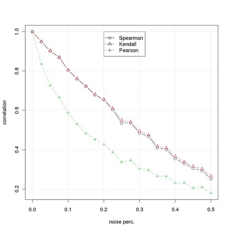
The estimates of correlation based on the Spearman and Kendall coefficient also exhibit a reduced noise sensitivity, a fact that we can check with the following code snippet:

1   eye    <- ia.get(face, animask(38,89,44,33))
2   ns     <- seq(0,0.5,0.025)
3   n      <- length(ns)
4   cvs    <- array(0, dim = c(n, 4))
5   S      <- 5
6   for(i in 1:n) {
7 ...     cvs[i,1] <- ns[i]
8 ...     for(s in 1:S) {
9 ...       neye     <- tm.addNoise(eye, "saltpepper", scale=255,
10 ...                               clipRange=c(0L, 255L), percent = ns[i])
11 ...       cvs[i,2] <- cvs[i,2] + cor(as.real(eye@data), as.real(neye@data),
12 ...                                  method="spearman")
13 ...       cvs[i,3] <- cvs[i,3] + cor(as.real(eye@data), as.real(neye@data),
14 ...                                  method="kendall")
15 ...       cvs[i,4] <- cvs[i,4] + cor(as.real(eye@data), as.real(neye@data),
16 ...                                  method="pearson")
17 ...     }
18 ...   }
19   cvs[,2] <- cvs[,2]/S
20   cvs[,3] <- cvs[,3]/S
21   cvs[,4] <- cvs[,4]/S

1 tm.dev("figures/ordinalRobustness")
2  matplot(cvs[,1], cvs[,2:4], pch=1:3, lty=1:3, type="b",
3 ...          xlab="noise perc.", ylab="correlation")
4  legend(0.2,1, c("Spearman", "Kendall", "Pearson"), lty=1:3, pch=1:3)
5  grid()
6 dev.off()

Figure 5.2:

The ordinal correlation estimates from the Spearman and Kendall coefficients are less sensitive to noise than the estimate provided by the Pearson coeffcient. The robustness of the Spearman and Kendall estimates, at least in the present case, is very similar suggesting the usage of the Spearman coefficient whose computation is much faster.

[next] [prev] [prev-tail] [front] [up]