1.2 Basic template matching

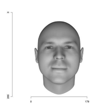
Template matching is the generic name for a set of techniques that quantify the similarity of two digital images, or portion thereof, in order to establish whether they are the same or not. Digital images are commonly represented with numerical arrays: monochrome images require a single matrix while color images require multiple matrices, one per color component. We will restrict our attention to monochrome images. Digital images can be stored in various formats such as jpeg, tiff, or ppm. A variant of the latter, specific to grey level images, is commonly identified with a .pgm suffix. Package AnImAl provides convenient functions to read them:

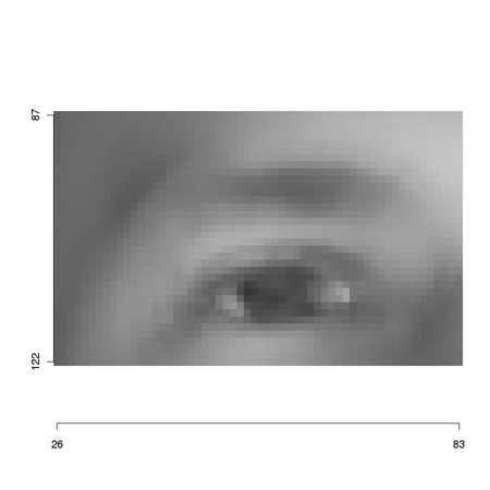
Note the darker region: it identifies R output. The coordinate system most often associated to an image is left-handed: the value of the x coordinate increases from left to right while that of the y coordinate increases from top to bottom (see Figure 1.1). This is due to images being stored as arrays and to the fact that the y coordinate is associated to the row number. R provides extensive graphical facilities and function tm.ploteps can be used to turn their output to postscript files:

Setting tm.plot.defaultFormat <- "X11" (uncommenting line 1 above) makes subsequent calls to tm.plot use the windowing system. We will routinely use tm.plot to produce the images inserted in this manual.

Figure 1.1: A sample monochrome image with its left-handed coordinate system.

The existence of an image coordinate system allows us to specify in a compact way rectangular regions: we simply need to provide the coordinates (x₀,y₀) of its upper left corner and the horizontal and vertical dimensions (dx,dy):

The result, reported in Figure 1.2, is a new, smaller image that carries on the knowledge of its original placement as the axes values show.

Figure 1.2: A detail of Figure 1.1: let us note that the coordinates in the original image are preserved.

As clarified in Figure TM1.2, the search for a template, such as the one presented in Figure 1.2, within an image, such as the one in Figure 1.1, is performed by scanning the whole image, extracting at each image position a region of interest whose size corresponds to that of the template:

Function ia.show in line 4 of the above code snippet would show image portion w in a window. However, what we need to do is to compare each image w to the reference template eye1 assessing their similarity. We should also store the resulting values in a map so that we can access them freely after the computation is completed.

Codelet 1 Basic template matching (./R/tm.basicTemplateMatching.R)
____________________________________________________________________________________________________________

This function illustrates the most basic template matching technique: the template is moved over each image position and the sum of the squared difference of aligned image and template pixels is considered an indicator of template dissimilarity.

1tm.basicTemplateMatching <- function(image, template) {

The first step is to get the linear dimensions of the template

2  dx <- ia.mask(template)@w 
3  dy <- ia.mask(template)@h

We then determine the extent of the image region of interest over which we need to slide our template

4  x0 <- ia.xmin(image) 
5  y0 <- ia.ymin(image) 
6  x1 <- ia.xmax(image) - dx 
7  y1 <- ia.ymax(image) - dy

This allows us to prepare the storage for the similarity scores

8  scores <- animage(array(0,dim=c(y1-y0+1,x1-x0+1)),storage="real",focus=image@focus)

and to perform the actual computation loop,

9  for(y in y0:y1) { 
10    for(x in x0:x1) {

sliding along each row and extracting in turn an image portion matching the size of the template

11      w <- ia.get(image, animask(x, y, dx, dy))

We modify the template so that it overlaps the extracted region

12      template@focus <- w@focus

and compute (and store) the matching score

13      scores[y,x] <- sum(ia.matop(function(x,y) (x-y)**2, w, template)@data) 
14    } 
15  }

We can finally return the image representing the similarity map

16  scores 
17}

______________________________________________________________________________________

It is now easy to spot our template in the image:

Note that the position of the template differs from that of the original eye1 as we down-sampled the image: the coordinates are halved. We can also have a look at the resulting matrices to get an idea of how extremal the matching value at the correct position is: this is related to the concept of signal to noise ratio that we will consider in depth in later chapters.

Figure 1.3: The distance map (left) and the similarity map (right) corresponding to the matching of template eye1 to face1.

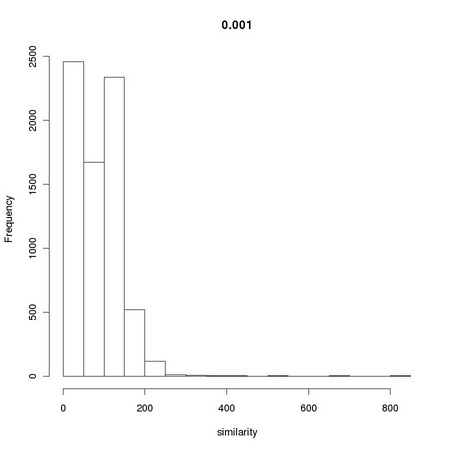
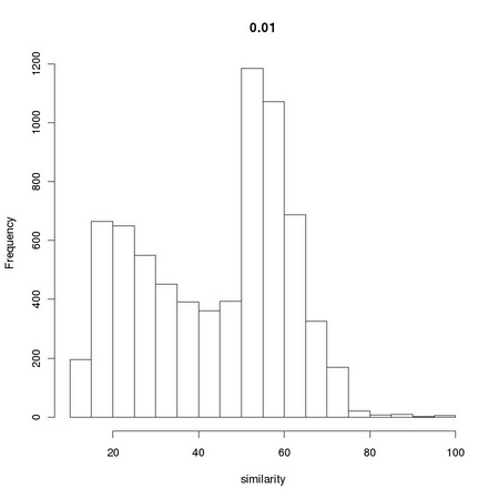
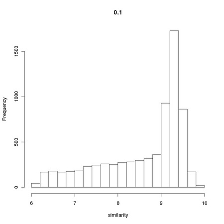
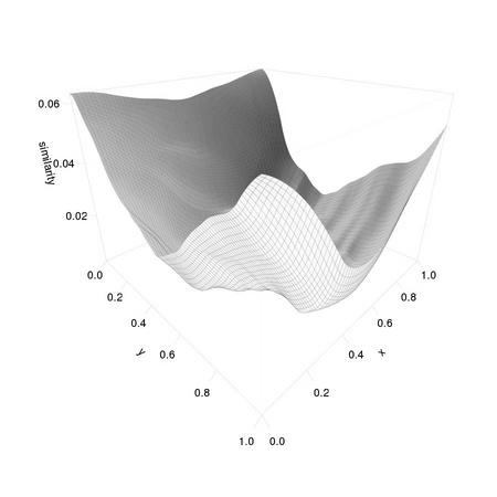
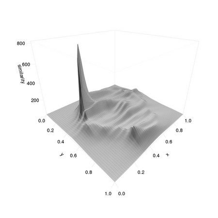
AnImAl provides ia.correlation, a faster and more flexible function to perform the task that will be considered in Chapter 3. Changing the value 0.001 used in the computation of simScores significantly affects the distribution of values:

The resulting distributions are reported in Figure 1.4.

Figure 1.4: The distributions of similarity scores obtained varying the denominator constant, 0.001, 0.01, 0.1 respectively from left to right. The highest similarity value determines the x range: the lower the value used in the normalization, the higher the dynamic range exhibited by the scores and the more far apart the value corresponding to the correct position from the remaining ones.