Log-polar imaging

Fondazione Bruno Kessler - Technologies of Vision

contains material from
Template Matching Techniques in Computer Vision: Theory and Practice
Roberto Brunelli © 2009 John Wiley & Sons, Ltd

[prev] [prev-tail] [tail] [up]

2.6 Log-polar imaging

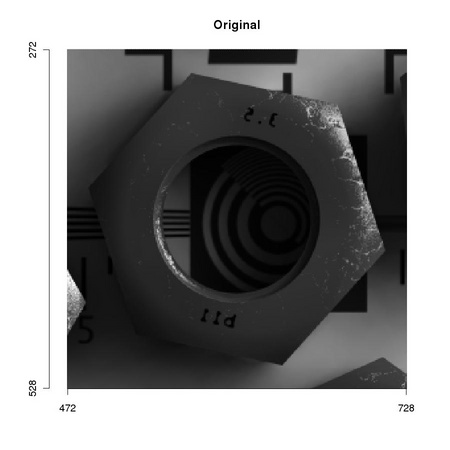
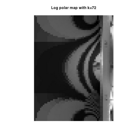
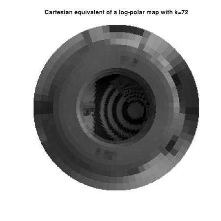
While the representation of image as rectangular arrays is the most widespread, alternative exists. Log-polar mapping, described in Section TM:2.4 is an example of space variant representation providing a spatial resolution decreasing from the center towards the boundary.

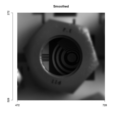
Log-polar mapping is usually obtained with specific sensors but can also be simulated via software to appreciate some of its characteristics. When we change the image representation from a (standard) rectangular lattice to a log-polar spatio-variant structure we are effectively performing a resampling task which is prone to aliasing if frequency content is not properly tuned. As log-polar sensor resolution is spatio-variant so must be the amount of smoothing applied before resampling. Usually, the two sensing structures are compared for a given maximum spatial resolution. In the case of a rectangular sensor the maximum resolution extends over the whole sensor while in the case of a log-polar sensor it is confined to the central (foveal) region.

1 # We select an image portion
2 #
3 A <- ia.get(i_orthoRed, animask(472,272,257,257))
4 tm.plot("figures/lpOrig", ia.show(A, main="Original"))
5 #
6 # and we smooth it, increasingly so towards the perifery,
7 # preparing it for a log-polar mapping with an angular
8 # resolution of 72 cells
9 #
10 sA <- tm.logPolarSmoothing(A, angularResolution = 72)
11 tm.plot("figures/lpSmooth", ia.show(sA, main="Smoothed"))
12 #
13 # and project/back project to get a feeling of the log-polar mapping with
14 # 3960 pixels instead of 51471
15 #
16 lpeA      <- tm.logPolarMapEquivalent(sA, R = 128, 72)
17 #
18 # We now create the 'real' log-polar map where the horizontal
19 # coordinate corresponds to rings, while the vertical one
20 # represents the angular 'sector'
21 #
22 lpmA      <- tm.logPolarMap(sA, 128, angularResolution = 72)
23 #
24 # and we plot it with a gamma correction of 2.2
25 #
26 tm.plot("figures/lpMap",
27 ...    plot(pixmapGrey((lpmA)**(1.0/2.2)),
28 ...    main="Log polar map with k=72"))
29 #
30 # comparing it to the cartesian back projection
31 # (with a gamma correction of 2.2)
32 #
33 tm.plot("figures/lpEquiv",
34 ...    plot(pixmapGrey((lpeA@data)**(1.0/2.2)),
35 ...    main="Cartesian equivalent of a log-polar map with k=72"))

Figure 2.9:

Log-polar mapping, providing image representation with spatio-variant resolution, requires a complex smoothing pre-processing. The images in the bottom row present the resulting map (left) and its back-projection in the standard image representation.

[prev] [prev-tail] [front] [up]