3.1 The ROC curve

A binary classification task can be considered as a binary hypothesis testin problem where one of the two competing hypotheses H₀ and H₁ must hold. The two basic probabilities characterizing the Neyman-Pearson approach to testing are the false alarm error probability P_F and the detection probability P_D. The former is the probability of returning H₁ when the true world state is described by H₀ and is also known as the probability of a type I error (or false acceptance rate, FAR). The latter, also known as the test power, gives the probability with which H₁ is returned (by the classifier) when the true world state is H₁. Neyman-Pearson classification, which maximizes P_D under a specified bound on P_F , results in a simple thresholding operation on the likelihood ratio value Λ() for a pattern under hypothesis H₀:

(3.1)

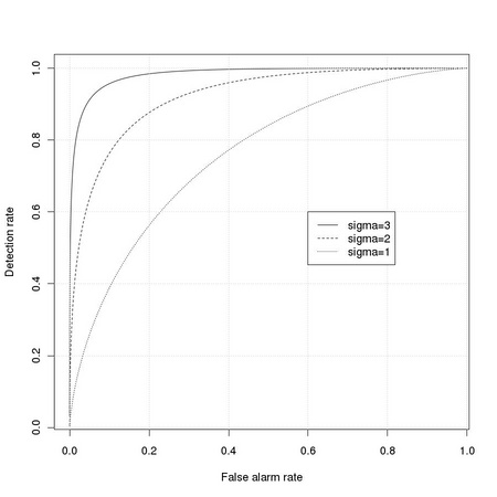
The relation between the two probabilities, specifically P_D as a function of P_F , is usually represented with a receiver operating characteristic (ROC) curve that is extensively discussed in Appendix TM:C:

(3.2)

The quantity 1 - P_D represents the false negative error probability and is also known as the false rejection rate (FRR). The ROC curve is often reported as

(3.3)

While the ROC curve provides detailed information on the trade-off between the two types of errors, classification system are often synthetically characterized by means of the equal error rate (EER), the intersection of the ROC curve with the diagonal

(3.4)

When the data distribution under the two competing hypotheses is Gaussian with the same covariance matrix (and different means) the probabilities considered above can be computed in close form (see Section TM:3.3) and the multidimensional case does not present significant differences from the one dimensional one. The key parameter, fixing the maximum achieavable performance, is the separation of the distributions mean with respect to distribution standard deviation. With reference to Equations TM:3.50-58, we can from parameter ν to

(3.5)

in order to compute P_D = P_D(P_F ) exploint the fact that the Q-function is simply the complement to 1 of the distribution function (pnorm)

Figure 3.1: When data are normally distributed the maximum achievable performance is determined by the separation of the classes relative to the standard deviation of the distribution σ0: the higher σ0, the closer to the upper left corner the curve.