|
Fondazione Bruno Kessler - Technologies of Vision
contains material from
Template Matching Techniques in Computer Vision: Theory and Practice
Roberto Brunelli © 2009 John Wiley & Sons, Ltd
The use of the normalized correlation coefficient allows us to cope with global linear intensity remapping of the images being compared.
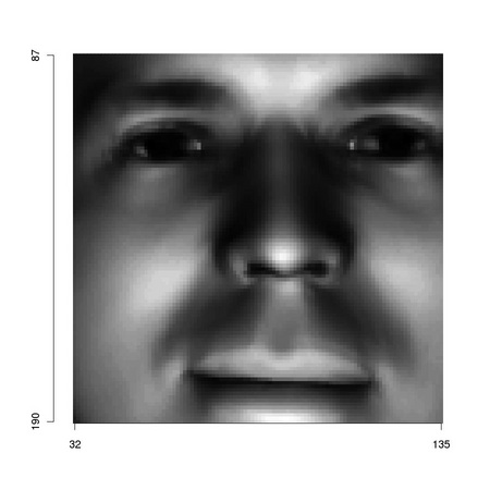
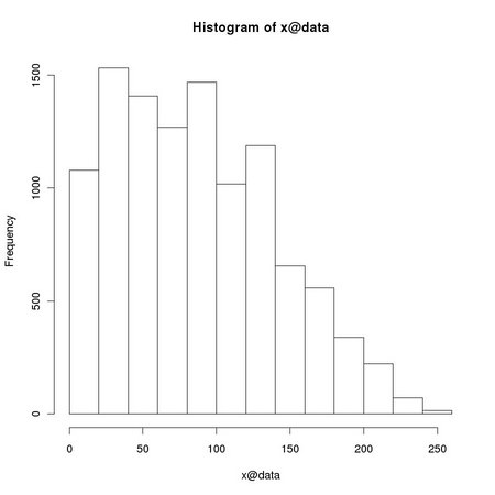
However, in many cases, image intensity undergoes a non linear transformation, a typical case being that of gamma correction, routinely applied by cameras in order to provide images that are more readable from human inspectors. The following code snippet applies a darkening gamma correction:
If we compute the correlation between dark and face we do not get 1 but a lower value
even if the value is not as low as one would expect by the perceived image difference. Let us consider the following problem: given a set of face images, snapped under different illumination conditions, we want to compare each of them to every other one. This means that for each comparison, the two images may be characterized by two different illumination conditions. A possible solution is to equalize in turn one of the images, the one whose histogram has a lower entropy and hence less information, so that it approximates the histogram of the more informative image. By doing so, we ensure that we do not throw away information. Let us assume that we are working with 8 bits images (256 intensity levels).
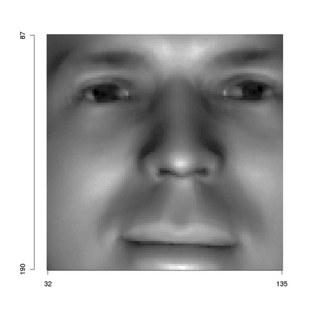
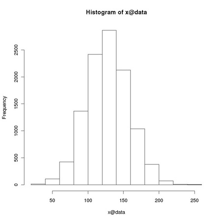
As face has a higher entropy, we equalize dark using as target histogra the histogram of face:
The histogram of darkEq is now very similar to that of face and the correlation value of the two images is higher than that of the couple (dark, face). The major drawback of this strategy is that every time we compare two (different) images we must perform a different equalization. An alternative is to choose a neutral equalization target, and normalize each image towards it. A natural choice is to choose a Gaussian distribution whose location paramters is 128 and whose standard deviation is such that no shadow or highlight clipping occurs when restricting to the interval [0.255]:
Even in this case we get a better correlation value than the one we got when comparing directly dark and face:
|