2.3 Noise

Images are often corrupted by noise, random fluctuations that can be characterized by their probability distribution. Two distributions are commonly used to model noise processes: the Gaussian (normal) distribution and the uniform distribution. While several noise processes affecting digital images can be described well by these distributions, quantum nature of light results in a different kind of noise, photon noise, following a Poisson distribution (see Section TM:2.1.4).

Codelet 2 Digital camera photon noise (../TeMa/R/tm.photonNoise.R)
____________________________________________________________________________________________________________

Quantum nature of light manifests itself as a Poisson noise affecting digital imaging. In order to simulate this noise process correctly we need to now a few parameters: the maximum number of electrons that fit within a pixel well and the corresponding ISO sensitivity, the ISO sensitivity at which the picture is taken, the maximum intensity value, and the gamma correction factor if any. These data allow us to map an intensity value in the digital image into and absolute number of electrons which is proportional to the number of photons. The latter provides the (single) parameter λ controlling the Poisson process. The default fullWell value is typical of a high-end digital reflex camera

1tm.photonNoise <- function(x, 
2                           maxValue        =   255, 
3                           gammaCorrection =   (1.0 / 2.2), 
4                           fullWell        = 51400, 
5                           fullWellIso     =   100, 
6                           iso             =   200) 
7  {

The first step is mapping the intensity value into a number proportional to the number of photons:

8    lambdaOrig      <- ((x/maxValue)**(1.0/gammaCorrection) 
9                        * fullWell 
10                        * (fullWellIso / iso))

A new, noisy value is generated according to the corresponding Poisson distribution:

11    lambdaPerturbed <- rpois(1, lambdaOrig)

and it is mapped back the digital image context

12    return(maxValue 
13           * ((lambdaPerturbed*(iso/fullWellIso))/fullWell)**gammaCorrection)

14  }

______________________________________________________________________________________

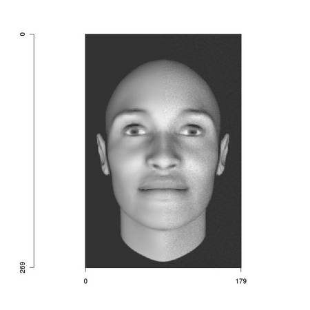
Photon noise is (proportionally) more significant in the darker areas of images: we choose a new sample image with a dark background and we apply to it a plausible amount of photon noise for a high ISO value of 3200 (the scale parameter of function tm.addNoise).

We can visually appreciate the effect of noise with a simple compositing operation:

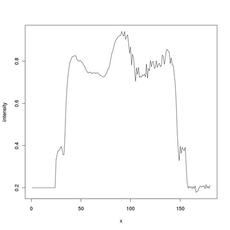
and having a detailed look at a sample row of the image

Figure 2.4: Photon noise is due to the quantum nature of light: as its variance is proportional to the square root of the average number of photons, its relative impact can be reduced by increasing the average number of photons, e.g. using large pixels.