Fondazione Bruno Kessler - Technologies of Vision
contains material from
Template Matching Techniques in Computer Vision: Theory and Practice
Roberto Brunelli © 2009 John Wiley & Sons, Ltd
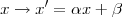
The basic template matching algorithm described in Chapter 1 is (very) sensitive to some commonly encountered template variations. When taking a digital image of a scene with a digital camera, even if we constrain ourselves to a fixed focal length, position and orientation, we have some remaining degrees of freedom, such as exposure time and focusing distance. We briefly consider the former: if we increase the exposure time (and the scene is relatively static) the result will be a lighter image. More photons are captured by the sensor and the reported intensity value will be proportionally higher. Additionally, sometimes, in order to make better use of the dynamic range available for image representation, the actual intensity values are streteched to fill a larger interval. The resulting transformation is of the following type
|
| (3.6) |
These transformations can be easily simulated:
We can modify the basic template matching of the previous chapter computing instead the following similarity measure
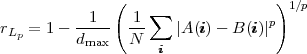 | (3.7) |
where A, and B are two congruent patterns and dmax is the maximum possible distance between them. This is exactly what ia.correlation does when invoked with type = "Lp" and normalize = FALSE:
The low contrast eye template is correctly locate in the low contrast face (let us note that which acts on array whose indices start from 1 while image indices, in this case, start from 0). However, if we try to locate the eye in the normal contrast image we see that the returned positio is not correct:
The problem can be solved by normalizing each image window to zero average and unit standard deviation before comparing it to the similarly normalized template:
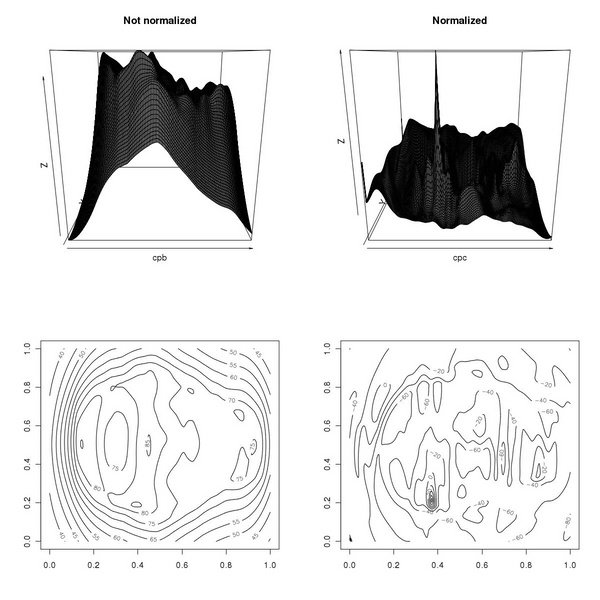
The normalization procedure let us spot the template correctly. The difference between the similarity measure obtained with the normalized/unnormalized Lp similarity measure can be appreciated by inspecting the contour plot of the corresponding maps: