Fondazione Bruno Kessler - Technologies of Vision

contains material from
Template Matching Techniques in Computer Vision: Theory and Practice
Roberto Brunelli © 2009 John Wiley & Sons, Ltd

3.3 Stein estimation

As discussed at length in Chapter TM:3, an accurate estimate of probability distributions is key to successfull hypotheses testing in general and template matching in particular. Even when coping with the simple case of normally distributed patterns, the estimation of the correct probability distribution parameter from experimentally avaialble data poses some challenges. The key quantity to be estimated in this case is the covariance matrix, which, together with the mean, completely characterize the distribution.

Codelet 4 On covariance estimation errors (R/tm.covarianceImpact.R)
____________________________________________________________________________________________________________

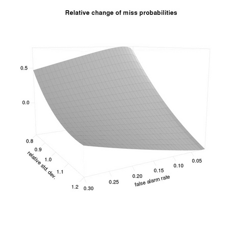
We want to visualize the impact of errors in the estimation of the covariance matrix on PD, the detection probability, at different operating conditions PF, as typical in the Neyman-Pearson paradigm. We refer to a single dimensional case, assuming that the distance of class means is 1: the difficulty of the problem is changed by changing the (common) standard deviation σ describing the two distributions. As easily checked from the results of Section TM3.3, we have that σ0 = σ-1. We want to compute the impact on PD(σ0) given that we set the operating condition using PF(σ), where σis our estimate of σ0 We first need to define a few functions, corresponding to Equation TM:3.15,

1tm.Q <- function(x, sd = 1.0) { 
2  1 - pnorm(x/sd) 
3}

to Equation TM:3.57,

4tm.Pf <- function(nu, sd0 = 1.0) { 
5  tm.Q(nu / sd0 + sd0/2) 
6}

and to Equation TM:3.58,

7tm.Pd <- function(nu, sd0 = 1.0) { 
8  tm.Q(nu / sd0 - sd0/2) 
9}

By choosing σ = 13, from which σ0 = 3, we get a reasonable testing case:

10tm.covarianceImpact <- function(sigma0 = 3,

We then consider PF ∈ [0.01, 0.3]

11                                pfRange = c(0.01, 0.3, 0.01),

and a moderately large range for σ= ασ0 α ∈ [0.8, 1.2]:

12                                pcRange = c(0.8, 1.2, 0.025)) {

We generate the sampling sequences:

13  ats <- seq(-3*sigma0, 3*sigma0, 0.1) 
14  pfs <- do.call(seq, as.list(pfRange)) 
15  pcs <- do.call(seq, as.list(pcRange)) * sigma0

and determine their lengths

16  npfs <- length(pfs) 
17  npcs <- length(pcs)

from which we appropriately size the map:

18  ci <- array(0, dim=c(npfs, npcs))

We now hypothesize several estimated values σ,

19  for(c in 1:npcs) {

and for each of them, we build the function nu ν = ν(x) : PF(ν) = x:

20    nu  <- splinefun(tm.Pf(ats, sd0=pcs[c]), ats) 
21    for(f in 1:npfs) {

We can now compute for a selected subset of operating conditions PF(σ) based on our estimated standard deviation, the difference in the miss probability with respect to the correct one PD(σ0):

22      ci[f,c] <- (1-tm.Pd(nu(pfs[f]), pcs[c])) /(1-tm.Pd(nu(pfs[f]), sigma0))-1 
23    } 
24  } 
25  list(pfs, pcs, ci) 
26}

______________________________________________________________________________________

1  source("R/tm.covarianceImpact.R") 
2  sigma0 <- 3 
3  ci     <- tm.covarianceImpact(sigma0) 
4  tm.dev("figures/covarianceImpact") 
5  persp(ci[[1]], ci[[2]]/sigma0, ci[[3]], theta = 150, phi = 10, 
6 ...         shade = 0.9, expand = 0.75, r = 3, lwd=0.1, 
7 ...         ticktype="detailed",cex=0.5, tcl=-0.5, 
8 ...         xlab="false alarm rate", ylab="relative std. dev.", 
9 ...         main="Relative change of miss probabilities", zlab="") 
10  dev.off()


PIC

Figure 3.3: Small errors in the estimation of the parameters of the probability ditributions can have a significant impact on classification performance. The plot shows how the error in the estimation of the standard deviation of normally distributed data results in an amplified detection error.


1 # load support for shrinkage covariance estimation 
2 # 
3 require(corpcor) 
4 # 
5 source("R/tm.shrinkageAdvantage.R") 
6 # the number of samples 
7 ns <- c(4,8,16,32,64,128,256,512) 
8 # the sample space dimension 
9 ps <- c(4,8,16,32,64,128,256,512) 
10 # 
11 shr <- tm.shrinkageAdvantage(ps, ns, ne = 10, ss = 10) 
12 # 
13 tm.dev("figures/shrinkageAdvantage") 
14 # 
15 persp(ns, ps, log(shr[[1]]/shr[[2]]), 
16 ...       theta = 50,  phi = -10, shade = 0.5, 
17 ...       ticktype="detailed", xlab="n", ylab="p", 
18 ...       zlab="log(error Frobenius norm)", d=2) 
19 # 
20 dev.off()


PIC

Figure 3.4: Shrinkage covariance estimation, based on the James-Stein insight, significantly outperforms the ordinary maximum likelihood estimator. The advantage increases with pattern space dimensionality p, and inversely to the number of samples.