4.1 Validity of distributional hypotheses
The discussion of template matching as hypothese testing presented in Chapter TM:3 focused on the
case of a deterministic signal corrupted by normal noise. The two hypotheses correspond to the case of
a deterministic signal corrupted by normal noise and pure normal noise. What happens when we
compare slightly displaced versions of the signal? In this case we are not comparing signal (possibly
plus noise) with noise, but signal with signal, albeit displaced. What kind of distribution can we
expect?
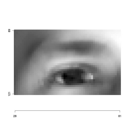
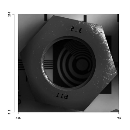
We will experimentally investigate this using two different templates: an eye and a hex nut (see
Figure 4.1).
1 sampleimages <- file.path(system.file(package="TeMa"), 2 ... "sampleimages") 3 # 4 img1 <- ia.scale(as.animage(getChannels(read.pnm( 5 ... file.path(sampleimages, "sampleFace_01.pgm")))), 6 ... 255) 7 m1 <- animask(28,89,54,33) 8 # 9 img2 <- ia.scale( 10 ... ia.readAnimage( 11 ... file.path(sampleimages, 12 ... "cameraSimulation", 13 ... "ortho_iso12233_large.tif")), 14 ... maxValue = 255)[[1]] 15 m2 <- animask(485,288,231,225) 16 # 17 tm.plot("figures/detail1", ia.show(ia.get(img1,m1))) 18 tm.plot("figures/detail2", ia.show(ia.get(img2,m2)))
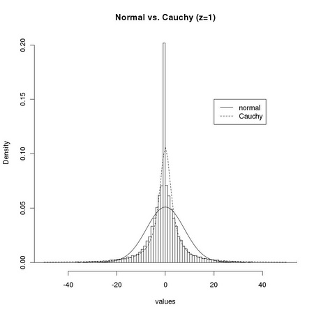
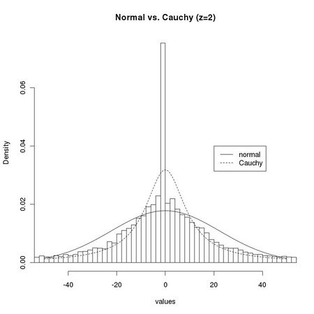
1 # We first focus on the effect of pattern misalignment: 2 # we consider the distributions of pixel values arising 3 # from displacing the patterns by a (Manhattan) distance 4 # z=1 and z=2 5 # 6 # 7 dtl <- ia.get(img1, m1) 8 img <- img1 9 m <- m1 10 # 11 z <- 1 12 values <- c() 13 # 14 for (i in z*seq(-1,1,by=1)) { 15 ... for (j in z*seq(-1,1,by=1)) { 16 ... dimg <- ia.sub(ia.get(ia.slide(img, z*i, z*j), m), 17 ... dtl) 18 ... values <- c(as.real(dimg@data), values) 19 ... } 20 ... } 21 # 22 tm.dev("figures/dsts_1") 23 hist(values,breaks=100,freq=FALSE,xlim=c(-50,50), 24 ... main="Normal vs. Cauchy (z=1)") 25 lines(seq(-50,50),dnorm(seq(-50,50), sd=sqrt(var(values))), lty=1) 26 lines(seq(-50,50),dcauchy(seq(-50,50),scale=mad(values,constant=1)),lty=2) 27 legend(20,0.15, c("normal", "Cauchy"), lty=1:2) 28 dev.off() 29 # 30 z <- 2 31 values <- c() 32 # 33 for (i in z*seq(-1,1,by=1)) { 34 ... for (j in z*seq(-1,1,by=1)) { 35 ... dimg <- ia.sub(ia.get(ia.slide(img, z*i, z*j), m), 36 ... dtl) 37 ... values <- c(as.real(dimg@data), values) 38 ... } 39 ... } 40 # 41 tm.dev("figures/dsts_2") 42 hist(values,breaks=100,freq=FALSE,xlim=c(-50,50), 43 ... main="Normal vs. Cauchy (z=2)") 44 lines(seq(-50,50),dnorm(seq(-50,50), sd=sqrt(var(values))), lty=1) 45 lines(seq(-50,50),dcauchy(seq(-50,50),scale=mad(values,constant=1)),lty=2) 46 legend(20,0.04, c("normal", "Cauchy"), lty=1:2) 47 dev.off()
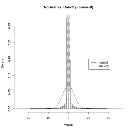
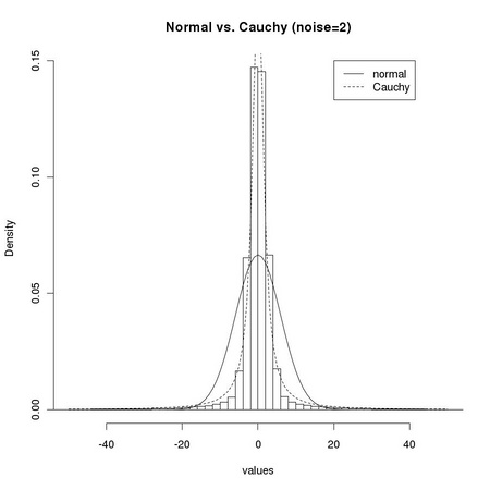
1 # We now consider a slightly different case: we consider 2 # a single displacement value z=1 (plus z=0) and change the 3 # amount of normal noise: noise=0 and noise=2 4 # 5 # 6 noise <- 0 7 img <- img2 8 m <- m2 9 dtl <- tm.addNoise(ia.get(img,m),"normal",scale=noise,clipRange=c(0,255)) 10 # 11 z <- 1 12 values <- c() 13 # 14 for (i in z*seq(-1,1,by=1)) { 15 ... for (j in z*seq(-1,1,by=1)) { 16 ... dimg <- ia.sub(tm.addNoise(ia.get(ia.slide(img, z*i, z*j), m), 17 ... "normal",scale=noise,clipRange=c(0,255)), 18 ... dtl) 19 ... values <- c(as.real(dimg@data), values) 20 ... } 21 ... } 22 # 23 tm.dev("figures/dsts_3") 24 hist(values,breaks=100,freq=FALSE,xlim=c(-50,50), 25 ... main="Normal vs. Cauchy (noise=0)") 26 lines(seq(-50,50),dnorm(seq(-50,50), sd=sqrt(var(values))), lty=1) 27 lines(seq(-50,50),dcauchy(seq(-50,50),scale=mad(values,constant=1)),lty=2) 28 legend(20,0.15, c("normal", "Cauchy"), lty=1:2) 29 dev.off() 30 # 31 noise <- 2 32 values <- c() 33 # 34 for (i in z*seq(-1,1,by=1)) { 35 ... for (j in z*seq(-1,1,by=1)) { 36 ... dimg <- ia.sub(tm.addNoise(ia.get(ia.slide(img, z*i, z*j), m), 37 ... "normal", scale=noise, clipRange=c(0,255)), 38 ... dtl) 39 ... values <- c(as.real(dimg@data), values) 40 ... } 41 ... } 42 # 43 tm.dev("figures/dsts_4") 44 hist(values,breaks=100,freq=FALSE,xlim=c(-50,50), 45 ... main="Normal vs. Cauchy (noise=2)") 46 lines(seq(-50,50),dnorm(seq(-50,50), sd=sqrt(var(values))), lty=1) 47 lines(seq(-50,50),dcauchy(seq(-50,50),scale=mad(values,constant=1)),lty=2) 48 legend(20,0.15, c("normal", "Cauchy"), lty=1:2) 49 dev.off()