Fondazione Bruno Kessler - Technologies of Vision

contains material from
Template Matching Techniques in Computer Vision: Theory and Practice
Roberto Brunelli © 2009 John Wiley & Sons, Ltd

4.2 Tanh estimators

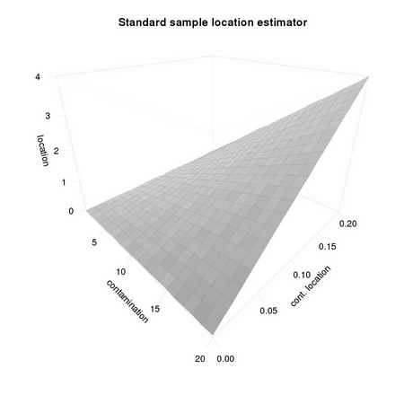
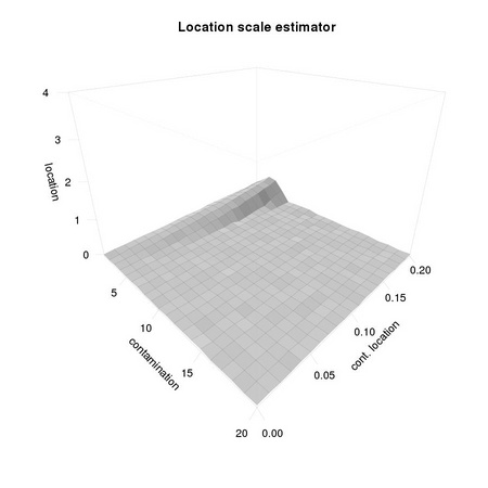
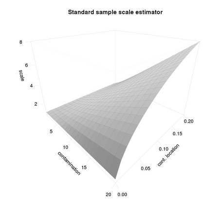
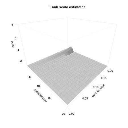
Deviations of the actual distribution from the expect (model) one have a profound impact on the resulting parameter estimates. The case we consider in the text, for small values of the contamination location paramter, can be considered as a model for the estimation of image normalization parameters in the context of face recognition. The distribution of face intensity values, while not necessarily Gaussian, could be fruitfully morphed to a normal distribution (we will consider this in the next chapter) and the perturbation considered is somehow similar to the presence of specularities, such as those often appearing at eyes.

1 values <- rnorm(100) 
2 ats    <- seq(1, 20, by=1) 
3 na     <- length(ats) 
4 cs     <- seq(0,  0.2, by=0.01) 
5 nc     <- length(cs) 
6 aveP   <- array(0, dim=c(na,nc)) 
7 sdP    <- array(0, dim=c(na,nc)) 
8 aveR   <- array(0, dim=c(na,nc)) 
9 sdR    <- array(0, dim=c(na,nc)) 
10 # 
11 cDist <- function(n=10000, c = 0.01, at=100) { 
12 ...  nm     <- as.integer(n*(1-c)) 
13 ...  array(c(rnorm(nm), rep(at, n-nm)), dim=c(n,1)) 
14 ... } 
15 # 
16 ic <- 0 
17 for(c in cs) { 
18 ...  ic <- ic+1 
19 ...  ia <- 0 
20 ...  for(a in ats) { 
21 ...   ia     <- ia+1 
22 ...   values <- cDist(c = c, at = a) 
23 ...   estP   <- tm.robustEstimates(values, "p") 
24 ...   estR   <- tm.robustEstimates(values, "O") 
25 ...   aveP[ia,ic] <- estP[1] ; sdP[ia,ic]  <- estP[2] 
26 ...   aveR[ia,ic] <- estR[1] ; sdR[ia,ic]  <- estR[2] 
27 ...  } 
28 ... } 
29 # 
30 tm.plot("figures/aveP", 
31 ...  persp(ats,cs,aveP,theta=45, phi=25,shade=0.35,expand=0.75,r = 1, 
32 ...       xlab="contamination", ylab="cont. location", 
33 ...       main="Standard sample location estimator", 
34 ...       zlim = c(min(min(aveR),min(aveP)),max(max(aveR),max(aveP))), 
35 ...       lwd=0.1, ticktype="detailed",zlab="location")) 
36 tm.plot("figures/aveR", 
37 ...  persp(ats,cs,aveR,theta=45, phi=25,shade=0.35,expand=0.75,r = 1, 
38 ...       xlab="contamination", ylab="cont. location", 
39 ...       main="Location scale estimator", 
40 ...       zlim = c(min(min(aveR),min(aveP)),max(max(aveR),max(aveP))), 
41 ...       lwd=0.1, ticktype="detailed",zlab="location")) 
42 tm.plot("figures/sdP", 
43 ...  persp(ats,cs,sdP,theta=45, phi=25,shade=0.35,expand=0.75,r = 1, 
44 ...       xlab="contamination", ylab="cont. location", 
45 ...       main="Standard sample scale estimator", 
46 ...       zlim = c(min(min(sdR),min(sdP)),max(max(sdR),max(sdP))), 
47 ...       lwd=0.1, ticktype="detailed",zlab="scale")) 
48 tm.plot("figures/sdR", 
49 ...  persp(ats,cs,sdR,theta=45, phi=25,shade=0.35,expand=0.75,r = 1, 
50 ...       xlab="contamination", ylab="cont. location", 
51 ...       main="Tanh scale estimator", 
52 ...       zlim = c(min(min(sdR),min(sdP)),max(max(sdR),max(sdP))), 
53 ...       lwd=0.1, ticktype="detailed",zlab="scale")) 
54 # 
55 tm.plot("figures/avePH",hist(aveP)) 
56 tm.plot("figures/aveRH",hist(aveR)) 
57 tm.plot("figures/sdPH", hist(sdP)) 
58 tm.plot("figures/sdRH", hist(sdR))


PIC PIC
PIC PIC

Figure 4.4: The plots make it clear that the standard sample estimators suffer significantly from the presence of contamination. The effect is more marked for the estimation of the scale parameter, a value that will turn out to be of paramount importance in many template matching techniques which rely on an accurate estimation of the covariance matrix.


PIC PIC
PIC PIC

Figure 4.5: This figures presents an alternative view of the data presented in Figure 4.4. We discarde the dependency on contamination value and location and we plot the histogram of the estimates in order to better appreciate the corresponding variability.


Tanh estimators can be used to define a robust version of the standard Pearson correlation coefficient as illustrated by function tm.robustifiedCorrelation.

Codelet 5 A simple approach to robustified correlation (../TeMa/R/tm.robustifiedCorrelation.R)
____________________________________________________________________________________________________________

Pearson correlation coefficient is closely related to the computation of the variance of a set of numbers: it is the dot product of two vectors previously normalized to zero average and unitary variance. The sensitivity of the standard sample variance estimator to the presences of outlying values, such as those due to salt and pepper noise, affects the robustness of the Pearson correlation coefficient. Equation TM:4.17 shows how we can define a robust correlation coefficient using a robust scale estimator. The function tm.robustifiedCorrelation implements Equation TM:4.17 using the scale estimates provided by tm.robustEstimates.

1tm.robustifiedCorrelation <- function(X, Y, mode="O") {

X and Y represent two images, usually normalized to zero location and unitary scale using tm.normalizeImage. The third parameter, mode, can assume three different values: "p", corresponding to the usual (non robust) sample estimator, "M", corresponding to a (non-refined) tanh estimator, and "O", corresponding to a one-step version of the tanh estimator. In order to exploit Equation TM:4.17, we must generate two new random variables that correspond respectively to the sum and to the difference of the two images:

2  XpY <- ia.add(X, Y) 
3  XmY <- ia.sub(X, Y)

proceeding to the computations required by Equation TM:4.17

4  sp  <- tm.robustEstimates(array(XpY@data, dim=c(ia.size(XpY),1)), mode) 
5  sm  <- tm.robustEstimates(array(XmY@data, dim=c(ia.size(XmY),1)), mode)
6  (sp[2]*sp[2] - sm[2]*sm[2])/ (sp[2]*sp[2] + sm[2]*sm[2]) 
7}

______________________________________________________________________________________