![[ N i ∑N i]
rB′N (α) = 1- (1 - α)max-i=1dm- + α--i=12d-m .
⌊N2 ⌋ ⌊N4 ⌋](tmCodeCompanion9x.png)
Fondazione Bruno Kessler - Technologies of Vision
contains material from
Template Matching Techniques in Computer Vision: Theory and Practice
Roberto Brunelli © 2009 John Wiley & Sons, Ltd
A simple and useful way to characterize the discriminatory power of a template matcher is to compute its signal to noise ratio SNR: its response at the correct location divided by its average response everywhere else. If the SNR is high, detection is expected to be reliable. We can detect our template simply by thresholding the response of the detector: small amounts of noise are not expected to make the value drop below threshold or making the value of other patterns arise above threshold. If the SNR is low, detection by thresholding might be unreliable or downright impossible. Function tm.snr provides a sample implementation of this quality parameter:
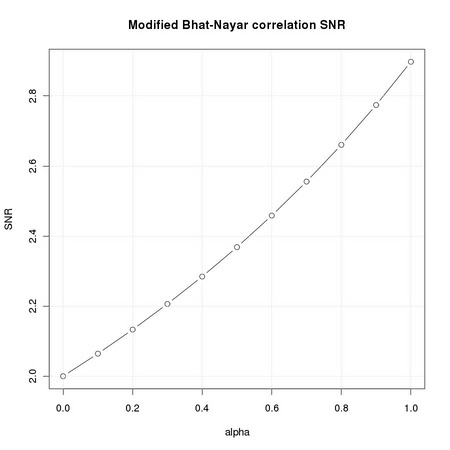
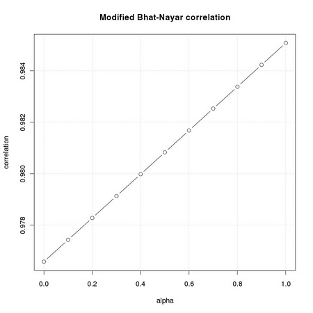
We can apply the concept of SNR to the comparison of the original Bhat-Nayar correlation measure (Equation TM:5.24) to the modified version Equation TM:5.27. The testbed we consider is that of matching a no-noise version of the eye region of the original face face image to a noisy version of the dark face. We compute the modified Bhat-Nayar correlation weighting the average part of the contribution with α:
|
| (5.1) |
When α = 0 we recover the original Bhat-Nayar definition, while α = 1 keeps only the average distance. In order to compute the SNR we must identify the reference template position: the image coordinates representing the upper left corner of the eye template, i.e. (38,89). Besides computing the signal to noise ratio, we want to check the actual correlation value returned at the reference template location.
As we can appreciate from the corresponding plots reported in Figure 5.3, the averaged version of the Bhat-Nayar distance exhibits a better SNR and a better correlation value.
|
The Bhat-Nayar similarity measure is an excellent example of the kind of robustness that we can achieve using ordinal similarity measures: monotone intensity transformation have no impact on the resulting estimates and noise effects are markedly reduced with respect to standard correlation: