Fondazione Bruno Kessler - Technologies of Vision

contains material from
Template Matching Techniques in Computer Vision: Theory and Practice
Roberto Brunelli © 2009 John Wiley & Sons, Ltd

5.4 Non Parametric Local Transforms

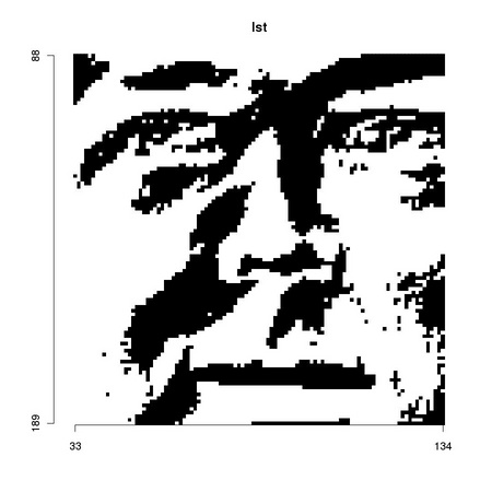
Another way to gain robustness to intensity transformations and small amounts of noise is by means of local image operations transforming intensity values into pseudo intensity values based on local rank information. The transformed values are then insensitive to positive monotone image mappings and can accomodate a small amount of noise as long as noise does not change the relative rank of the intensity values. We consider four different non parametric local transforms based on ordinal information:

  1. rank,
  2. census,
  3. modified census, including the central reference pixel,
  4. incremental sign transform.

All the above transforms are provided by function tm.ordinalTransform with the use of a proper mode selector value (see Figure 5.4. Let us note that, as the transform cannot be computed at the boundary of the image, function tm.ordinalTransform performs an autoframing operation by default: we can prevent it by using autoFrame=FALSE.

1 N8        <- tm.squareNeighborhood(1L) 
2 rankT     <- tm.ordinalTransform(face, N8, mode="rank") 
3 censusmT  <- tm.ordinalTransform(face, N8, mode="census") 
4 censusT   <- tm.ordinalTransform(face, N8, mode="censusm") 
5 istT      <- tm.ordinalTransform(face, N8, mode="ist") 
6 tm.plot("figures/rank",   ia.show(rankT,   main="Rank")) 
7 tm.plot("figures/census", ia.show(censusT, main="Census")) 
8 tm.plot("figures/censusm",ia.show(censusmT,main="Census (modified)")) 
9 tm.plot("figures/ist",    ia.show(istT,    main="Ist"))


PIC PIC
PIC PIC

Figure 5.4: The different images present the four non parametric local transforms considered in the text.


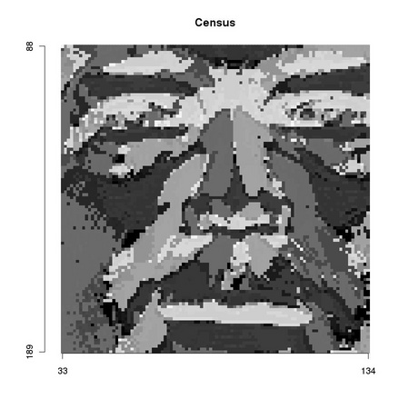
The neighborhood used for the computation of the local transforms is important for several reasons. The (computational) complexity of the transform depends on the number of points in the neighborhood. In the case of the census transform, the storage requirements for the result scale linearly with the number of points. As the result must be stored as an integer number for efficient use in image comparison tasks, the maximum number of points does not exceed 32 (sometimes 64). The number of points directly affects the dynamic range of the rank transform: the range corresponds to the number of points in the neighborhood, the larger, the more detailed the information provided.

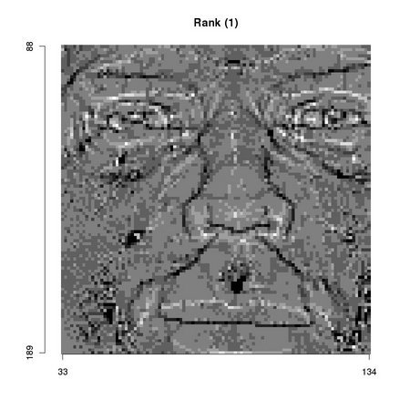
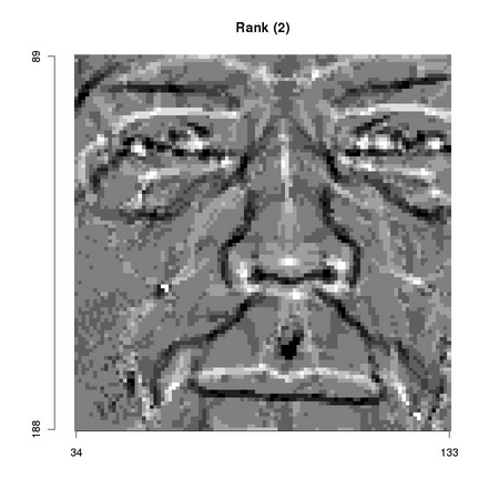
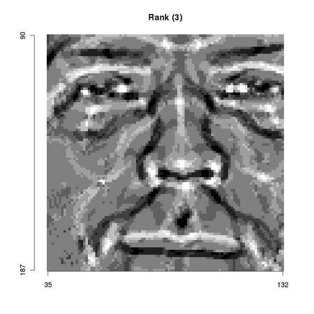
It is possible to keep the number of points in the neighborhood small while increasing their spacing. This operation has a beneficial effect as the relative ordering of the pixel intensity values becomes more stable with increasing spacing: for a given local gradient, the farther apart the pixels, the greater the difference, and the more stable the relative ranking. The phenomenon can be visually appreciated in Figure 5.5

1 rankT1     <- tm.ordinalTransform(face, N8,    mode="rank") 
2 rankT2     <- tm.ordinalTransform(face, N8*2L, mode="rank") 
3 rankT3     <- tm.ordinalTransform(face, N8*3L, mode="rank") 
4 tm.plot("figures/spacing1", ia.show(rankT1, main="Rank (1)")) 
5 tm.plot("figures/spacing2", ia.show(rankT2, main="Rank (2)")) 
6 tm.plot("figures/spacing3", ia.show(rankT3, main="Rank (3)"))


PIC PIC PIC

Figure 5.5: Increasing the spacing among the pixels of the neighborhood may increase the stability of the ordinal relations among the pixel intensity values with no impact on computation time or result storage requirements. The above images show what happens for the rank transform.


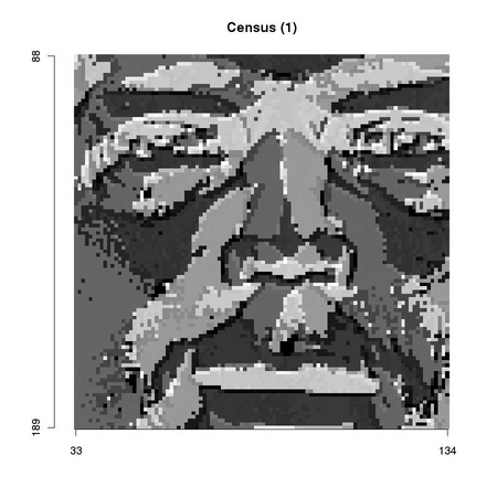
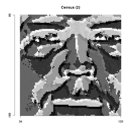
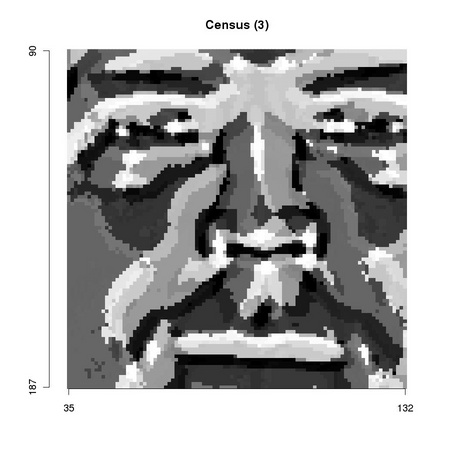
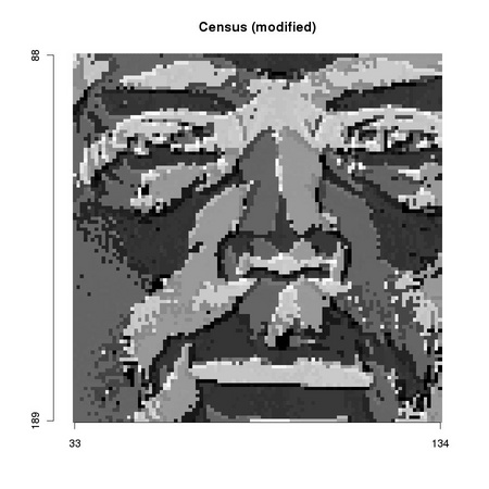
A similar effect can be observed for the census transform (see Figure 5.6).


PIC PIC PIC

Figure 5.6: The effect of neighborhood spacing on the result of the census transform.


1  # 
2  cs  <- seq(0,0.4,0.02) 
3  n   <- length(cs) 
4  res <- array(0, dim=c(n, 4)) 
5  i   <- 0 
6  X   <- tm.ordinalTransform(dark, N8, mode="census") 
7  for(c in cs) { 
8 ...    i        <- i + 1 
9 ...    res[i,1] <- c 
10 ...    # 
11 ...    Y <- tm.ordinalTransform(tm.addNoise(dark, noiseType="saltpepper", 
12 ...                                         scale = 255, clipRange=c(0L,255L), 
13 ...                                         percent=c), 
14 ...                                         N8, mode = "census") 
15 ...    # 
16 ...    res[i,2] <- tm.hamming(X, Y, width=8) 
17 ...    res[i,3] <- tm.tanimoto(X, Y) 
18 ...    res[i,4] <- tm.dixonKoehler(X, Y, width=8) 
19 ...  } 
20  # 
21 tm.dev("figures/bitDistances") 
22  matplot(res[,1], res[,2:4], type="b", pch=2:4, lty=2:4, 
23 ...          xlab="Salt&pepper contamination", ylab="Bit distance") 
24  legend(0.0,0.3,c("Hamming", "Tanimoto", "Dixon-Koehler"), lty=2:4, pch=2:4) 
25  grid() 
26 dev.off()


PIC

Figure 5.7: The correct way to compare the images resulting from the census transform is to use bit based distances. The plot illustrates the results obtained applying the distances dicussed in the text.