Fondazione Bruno Kessler - Technologies of Vision

contains material from
Template Matching Techniques in Computer Vision: Theory and Practice
Roberto Brunelli © 2009 John Wiley & Sons, Ltd

6.1 Maximizing SNR over class samples

In this section we start to address the problems arising from intrinsic signal variability. We no longer limit ourselves to the the problem of detecting a single, deterministic signal corrupted by noise, and we move to the problem of detecting a class of signals in the presence of noise. The signals we will consider are images of faces, a class of patterns of significant practical and theoretical interest. The dataset we will be using comprises 800 different faces, equally distributed over four differents races and the two genders.

1 basepath    <- "../theFaceDbs/races" 
2 racesImages <- scan(file.path(basepath, "racesImageNames"), list(""))[[1]] 
3 N           <- length(racesImages) 
4 m           <- animask(5,13,21,25) 
5 d                  <- 21*25 
6 raceSamples        <- c() 
7 raceSamplesMatrix  <- array(0, dim=c(N,d)) 
8 for(i in 1:N) { 
9 ...   img <- as.animage(getChannels(read.pnm(file.path(basepath, 
10 ...                                                   racesImages[[i]])))) 
11 ...   img <- ia.get(img, m) 
12 ...   raceSamples          <- c(img, raceSamples) 
13 ...   raceSamplesMatrix[i,] <- as.real(img@data) 
14 ... }

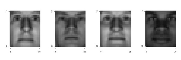
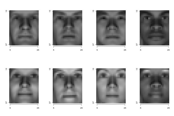
It is interesting to note the result of clustering the above data respectivel with 4 clusters, the number of races considered, and with 8 clusters the number of races times the number of genders:

1 kns <- list(2,4,6,8,10,12,14,16,18,20,22,24,26,28,30,32) 
2 kcs <- ia.map(function(n) sort(clara(raceSamplesMatrix,  n)$i.med), kns) 
3 k32 <- raceSamplesMatrix[kcs[[16]],]

The default metrics used by function clara is the Euclidean norm (L2) discussed in a previous chapter. Samples are regularly (consecutively) organized in groups of 200 items, 100 males and 100 females. The above clustering procedure, of which we reported the indices identifying each computed cluster within the original data, assigns 1 cluster center to each race (or race and gender) group.

1 tm.dev("figures/fourClusters", width=6, height=2) 
2 par(mfrow = c(1,4)) 
3 for(i in kcs[[2]]) { 
4 ... ia.show(raceSamples[[i]]) 
5 ... } 
6 dev.off() 
7 tm.dev("figures/eightClusters", width=6, height=4) 
8 par(mfcol = c(2,4)) 
9 for(i in kcs[[4]]) { 
10 ... ia.show(raceSamples[[i]]) 
11 ... } 
12 dev.off()


PIC

Figure 6.1: The images corresponding to the centers of the four cluster result. They belong to the four different racial groups, suggesting that the task of race discrimination can be effectively solved by template matching techniques using appropriately selected race prototypes.


PIC

Figure 6.2: The images corresponding to the centers of the eight cluster result. The remark of Figure 6.1 still applies. Interestingly, the upper row presents male samples, the lower row female examples: even the task of automatic gender determination seems to be solvable with template matching techniques. Chapter TM:12 addresses the race/gender discrimination problem using a couple of techniques related to template matching: regularization network and support vector machines.


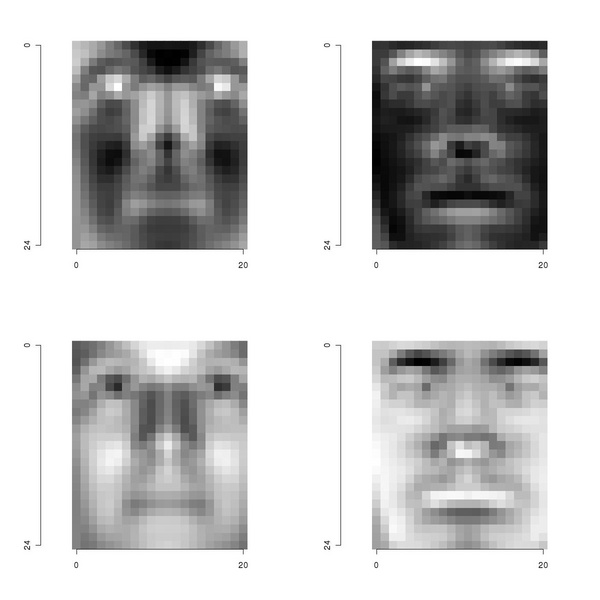
As detailed in Section TM:6.1, the optimal matched filter for the whole image set is given by the dominant eigenvector. Let us note that, in this case, the required covariance matrix is the not-centered one:

Σ =  XT X
(6.1)

where X is a matrix whose rows correspond to our face images, linearized as vectors:

1  var <- t(raceSamplesMatrix) %*% raceSamplesMatrix

The computation of the eigenvectors is straightforward:

1  evs <- eigen(var) 
2  # and we de-linearize the most significant twos 
3  # into an image 
4  ev1 <- as.animage(x <- array(evs$vectors[,1], dim=c(25,21))) 
5  ev2 <- as.animage(x <- array(evs$vectors[,2], dim=c(25,21))) 
6 tm.dev("figures/evs", width=6, height=6) 
7 par(mfcol = c(2,2)) 
8 ia.show(ev1) 
9 ia.show(ia.scale(ia.mult(ev1, -1))) 
10 ia.show(ev2) 
11 ia.show(ia.scale(ia.mult(ev2, -1))) 
12 dev.off()


PIC

Figure 6.3: The two most significant eigenvectors of the uncentered covariance matrix. The most significant one (first column to the left) resembles the average face. Let us note that there is an ambiguity on sign: the lower row contains the inverted version of the first row (returned as eigenvectors). In this case, we should use the inverted, most significant eigenvector as matched filter.