6.2 Multi-class Synthetic Discriminant Functions
Synthetic discriminant functions, SDFs for short, are introduced in Chapter TM:6.1 as a way to
generate a single direction onto which samples from a given set project (more or less) at the same,
predefined point. The construction of an SDF relies on the possibility of solving a linear set of
equations obtained by enforcing the projection values of a given set of patterns: the solution can be
expressed as a linear combination of the available samples. There are two related effects that we want
to explore:
- the distribution of the projection values obtained from patterns of the same class but not
explicitly used in building the SDF, and the dependency of its spread on the number of
sampels used in the SDF;
- how does an SDF compares with projection onto the (scaled) mean sample, both visually
and interms of the resulting distribution of projection values.
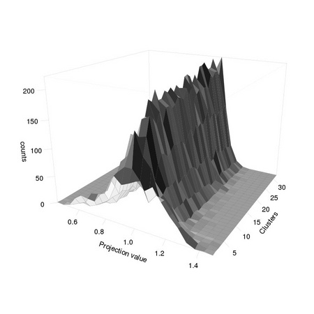
In order to investigate the first issue, we build a sequence of SDFs, using as building samples the
centers of an increasing number of clusters computed from the whole set of available faces (using
function clara from package cluster). We build a least squares SDF minimizing the projection error
onto the whole face dataset.
1 ks <- 1:32 2 breaks <- seq(0.4,1.5,0.05) 3 map <- array(0, dim=c(length(breaks)-1, length(ks))) 4 for(k in 1:length(ks)) { 5 ... sdf<-tm.sdf(t(clara(raceSamplesMatrix, ks[k])$medoids), 6 ... t(raceSamplesMatrix)) 7 ... map[,k]<-hist(raceSamplesMatrix %*% sdf,breaks=breaks,main=k)$counts 8 ... } 9 tm.dev("figures/sdfVsSamples") 10 persp(seq(0.425, 1.5, 0.05), 1:32, map, theta = 30, phi = 20, 11 ... shade = 0.7, expand = 0.75, r = 3, lwd=0.1, ylab="Clusters", 12 ... ticktype="detailed",cex=0.5,tcl=-0.5, xlab="Projection value",zlab="counts") 13 dev.off()
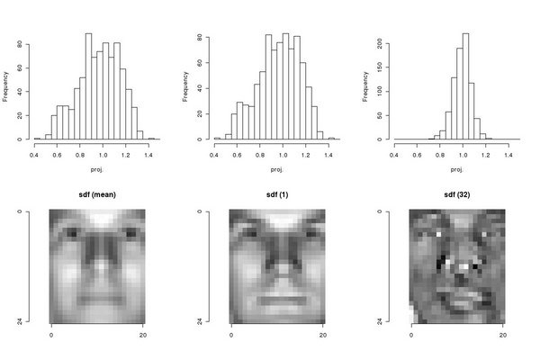
The second issue can be addressed in a straightforward way: we compute the average face, the least
squares SDF based on a single cluster description, and the least sqaures SDF based on a 32 cluster
description:
1 n <- dim(raceSamplesMatrix)[1] 2 mean <- raceSamplesMatrix[1,] 3 for(i in 2:n) 4 ... mean <- mean + raceSamplesMatrix[i,] 5 mean <-mean / n 6 sdf.m <-tm.sdf(t(matrix(mean, nrow=1)), t(raceSamplesMatrix)) 7 sdf.1 <-tm.sdf(t(clara(raceSamplesMatrix,1)$medoids),t(raceSamplesMatrix)) 8 sdf.32<-tm.sdf(t(clara(raceSamplesMatrix,32)$medoids),t(raceSamplesMatrix)) 9 # 10 tm.dev("figures/meanVsSdf", width=6, height=4) 11 par(mfrow = c(2,3)) 12 hist(raceSamplesMatrix %*% sdf.m, breaks=seq(0.4,1.5,0.05), 13 ... xlab="proj.", main="") 14 hist(raceSamplesMatrix %*% sdf.1, breaks=seq(0.4,1.5,0.05), 15 ... xlab="proj.", main="") 16 hist(raceSamplesMatrix %*% sdf.32, breaks=seq(0.4,1.5,0.05), 17 ... xlab="proj.", main="") 18 sdf.m.i <- as.animage(array(sdf.m, dim=c(25,21))) 19 sdf.1.i <- as.animage(array(sdf.1, dim=c(25,21))) 20 sdf.32.i <- as.animage(array(sdf.32, dim=c(25,21))) 21 ia.show(ia.scale(sdf.m.i),main="sdf (mean)") 22 ia.show(ia.scale(sdf.1.i),main="sdf (1)") 23 ia.show(ia.scale(sdf.32.i),main="sdf (32)") 24 dev.off()
As we can observe in Figure 6.5, the difference between sdf.m and sdf.1 is minor, but sdf.32
results in a significantly different filter providing superior performance. The dispersion of the
projection values around the required value (i.e. 1) can be easily quantified by computing the variance
of the values:
1 var(raceSamplesMatrix %*% sdf.m)
1 var(raceSamplesMatrix %*% sdf.1)
1 var(raceSamplesMatrix %*% sdf.32)
from which we see that there is almost an order of magnitude of difference.