Fondazione Bruno Kessler - Technologies of Vision

contains material from
Template Matching Techniques in Computer Vision: Theory and Practice
Roberto Brunelli © 2009 John Wiley & Sons, Ltd

7.1 Edge detection

Many patterns can be profitably represented by means of curves (as opposed to areas). Two new problems arise: how a reliable line based representation of a pattern can be obtained and how such representations can be exploited to efficiently find and compare patterns. In this section we describe a method to derive this kind of representations from a generic image, while the next sections will focus on how such a representation can be exploited to detect patterns in a robust and efficient way.

A basic way to obtain a line drawing from any image is to detect points of significant gradient intensity. The presence of noise makes the task more difficult as noise originates spurious intensity variations. In order to discriminate in a reliable way real gradients from noise originated ones we must have an estimate of the gradient intensity due to noise, and this is related to the amount of noise. In many cases the amount of noise itself is not known and we must estimate it from image data whose structure (distribution) is not necessarily known.

1 sampleimages <- file.path(system.file(package="TeMa"), 
2 ...                               "sampleimages") 
3 face         <- ia.scale(as.animage(getChannels(read.pnm( 
4 ...                   file.path(sampleimages, "sampleFace_01.pgm")))), 
5 ...                   255) 
6 face@outside <- 255 
7 nface        <- tm.addNoise(face, scale = 2.0, clipRange = c(0,255))

This is a good place where robust scale estimators can be profitably used. As Intermezzo TM:7.1 points out, we can get an estimate of noise standard deviation by computing the L2 norm of the convolution with a zero sum, unitary norm high pass filter kernel such as -1√ --
  2,1√--
 2:

1 sqrt( 
2 ...  var( 
3 ...   as.real( 
4 ...    ia.frame(ia.convolution(nface, 
5 ...                            array(c(0, -1/sqrt(2), 1/sqrt(2)),c(1,3))), 
6 ...             3)@data)))
1[1] 8.67417

but the returned value is way too high. The reason is that the image contains structure: it is not just a uniform value plus noise. However, at least in this specific case, we can consider the amount of image structure as a perturbation of a uniform surface as significant detail is restricted to a small percentage of the whole area. We can then use a robust scale estimator such as the mad to automatically get rid of it, obtaining a much more reliable estimate of the noise level:

1   mad(ia.frame(ia.convolution(nface,       array(c(0,      -1/sqrt(2), 
2 ...   1/sqrt(2)),c(1,3))), 3)@data)
1[1] 1.941272

that results in a much closer value. Function tm.estimateNoiseLevel relies on the above estimator. A simplified version of the method described in Section TM:7 is implemented by function tm.edgeDetection whose inner workings can be controlled by its several parameters.

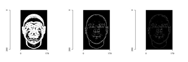
While thresholding gradient magnitude to get rid of spurious edges is necessary it is not sufficient as illustrated in Figure 7.1:

1 e1 <- tm.edgeDetection(nface,1,alpha=0.001, onlyFirstThr = TRUE) 
2 e2 <- tm.edgeDetection(nface,1,alpha=0.001, onlyFirstThr = FALSE) 
3 tm.dev("figures/edgeDetection1", width=6, height=2) 
4 par(mfrow = c(1,3)) 
5 ia.show(e1) 
6 ia.show(ia.greater(e2, 0)) 
7 ia.show(e2) 
8 dev.off()


PIC

Figure 7.1: Reliable edge detection must take into account non local information to get rid of spurious edges. The image to the left is generated by simple gradient threhsolding: too many pixels get classified as edges. The edge map to the right is computed taking into account the expected response of the second derivative at the pixels that pass the simple gradient intensity test. The analysis of the second derivative provides additional information: the spacing of the extrema is related to the blurring of the detected edges and can be exploited to further filter them, e.g. to create different edge maps representing different image structures. The intensity value of edge pixels is proportional to the second derivative extrema spacing.


1 e3 <- tm.edgeDetection(nface, 2,alpha=0.001, onlyFirstThr = FALSE) 
2 e4 <- tm.edgeDetection(nface, 4,alpha=0.001, onlyFirstThr = FALSE) 
3 e5 <- tm.edgeDetection(nface, 8,alpha=0.001, onlyFirstThr = FALSE) 
4 e6 <- tm.edgeDetection(nface,16,alpha=0.001, onlyFirstThr = FALSE) 
5 tm.dev("figures/edgeDetection2", width=6, height=6) 
6 par(mfrow = c(2,2)) 
7 ia.show(ia.greater(e3,0), main="Scale = 2") 
8 ia.show(ia.greater(e4,0), main="Scale = 4") 
9 ia.show(ia.greater(e5,0), main="Scale = 8") 
10 ia.show(ia.greater(e6,0), main="Scale = 16") 
11 dev.off()


PIC

Figure 7.2: The scale parameter of tm.edgeDetection allows us to investigate the edge structure at different scales, effectively exploring a resolution space.