Fondazione Bruno Kessler - Technologies of Vision

contains material from
Template Matching Techniques in Computer Vision: Theory and Practice
Roberto Brunelli © 2009 John Wiley & Sons, Ltd

7.2 The Hough Transform

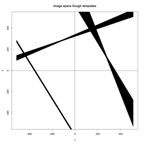
The Hough transform is an efficient way to perform template matching when the pixel representation of the templates is at the same time sparse (only a fraction of the pixels in the image are representative) and at the same time continuous so that local directional information can be used to focus the update of the cells in accumulator space. The equivalent template in image space can be obtained by backprojecting a single cell into image space.

The detailed shape of the resulting template is not obvious even in simple cases such as line detection using the normal parametrization (see Figure 7.3).

1 tm.dev("figures/houghImageSpaceLineTemplates", width=6, height=6) 
2 tm.houghImageSpaceClean() 
3 tm.houghLineCell(512, 300,tm.rad(20), 10,tm.rad(10),20) 
4 tm.houghLineCell(512, 300,tm.rad(110),10,tm.rad(5),20) 
5 tm.houghLineCell(512, 300,tm.rad(210),10,tm.rad(0.1),20) 
6 dev.off()


PIC

Figure 7.3: The finite extent of a cell in Hough space determines the image space region providing support to the corresponding accumulator. The image shows the image space templates resulting from the normal line representation for increasing angular resolution. The lower the angular resolution the more butterfly like the template.


1 img      <- animage(matrix(data = 0, nrow=33,ncol=33), storage = "real", 
2 ...                     focus = c(-16L,-16L)) 
3 noisyImg <- tm.addNoise(ia.mult(img, 0), noiseType="normal", scale=0.4) 
4 # 
5 # compute the standard Hough transform 
6 # 
7 h        <- tm.houghTransform(noisyImg, 33, 16, view = FALSE) 
8 # 
9 # and transform counts into probability 
10 # 
11 hmap     <- tm.mapHoughTransform(noisyImg, 33, 16, 0.4, view = FALSE) 
12 # 
13 tm.dev("figures/houghMap", width=6) 
14  tm.houghPlot(noisyImg, h, hmap) 
15 dev.off()


PIC

Figure 7.4: The accumulator provided by the Hough transform can be interpreted in a probabilistic way if the distribution of image noise is known. The figure shows the noisy image with a single line (left), the Hough accumulator (middle), and the resulting probability map (right).