Fondazione Bruno Kessler - Technologies of Vision

contains material from
Template Matching Techniques in Computer Vision: Theory and Practice
Roberto Brunelli © 2009 John Wiley & Sons, Ltd

8.1 Principal component analysis

One of the drawbacks of template matching is its high computational cost which is related to the resolution of the images being compared. It is then of interest finding a lower dimensionality representation that:

The most widely used transform satisfying the above constraints is principal component analysis (PCA): a translation and rotation of the original coordinate system, providing a set of directions sorted by decreasing contribution to pattern representation. It is a pattern specific representation that, in many cases of practical interest, allows us to use a limited subset of directions to approximate well the pattern. The better the require approximation, the higher the number of directions required.

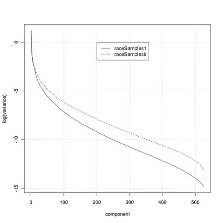
We now read a set of 800, geometrically normalized, grey images representing faces from multiple races. We then create two different vectorized sets, extracting the central face region (raceSample1) and an extended set with additional 8 congruent images at 1 pixel distance (raceSample9).

1 racesImages  <- scan("../theFaceDbs/races/imageNames", list(""))[[1]] 
2 raceSamples1 <- array(0, dim=c(800, 525)) 
3 raceSamples9 <- array(0, dim=c(800*9, 525)) 
4 # 
5 idx <- 0 
6 for(i in 1:800) { 
7 ...   a <- getChannels(read.pnm(paste("../theFaceDbs/races", racesImages[[i]], 
8 ...        sep="/"))) 
9 ...   raceSamples1[i,] <- ia.get(as.animage(a), animask(5,13,21,25))@data 
10 ...   for(dy in -1:1)  { 
11 ...     for(dx in -1:1) { 
12 ...       idx <- idx+1 
13 ...       raceSamples9[idx,] <- ia.get(as.animage(a), animask(5+dx,13+dy,21,25))@data 
14 ...     } 
15 ...   } 
16 ... }

We can now compute the covariance matrices and, using the singular value decomposition, determine its eigenvalues representing the variance described by each direction

1 mycov1 <- cov(raceSamples1) 
2 mysvd1 <- fast.svd(mycov1) 
3 mycov9 <- cov(raceSamples9) 
4 mysvd9 <- fast.svd(mycov9)

generating a comparative plot

1 tm.dev("figures/pca1") 
2 plot(log(mysvd1$d[1:525]), type="l", lty=1, xlab="component", ylab="log(variance)") 
3 lines(log(mysvd9$d[1:525]), type="l", lty=2, xlab="component", ylab="log(variance)") 
4 grid() 
5 legend(200, 0, c("raceSamples1", "raceSamples9"), lty=1:2) 
6 dev.off()


PIC

Figure 8.1: The variability of patterns impacts on the number of principal components required to approximate them well. The plot compares the two sets raceSamples1 and raceSamples9: as the variability of the latter is greater than that of the former, the variance captured by the principal directions decreases slowlier.


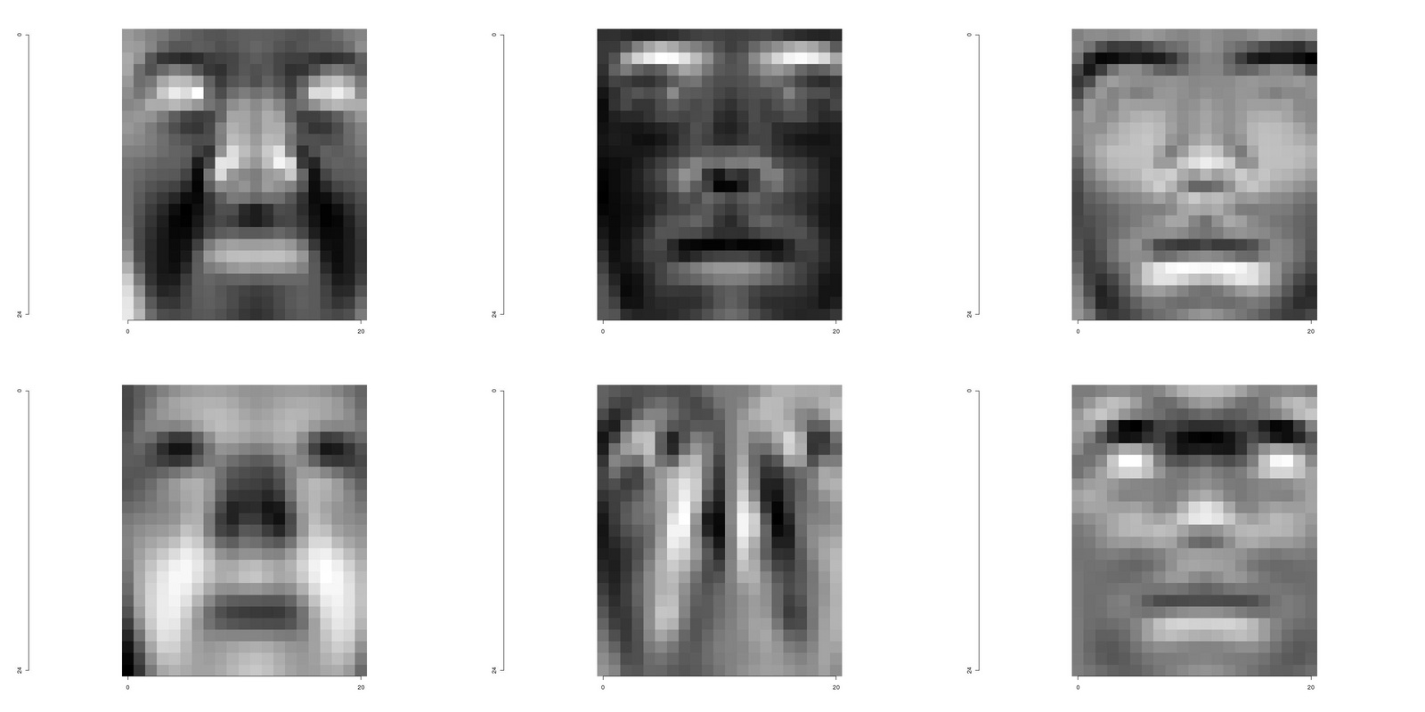
The eigenvectors, or eigenfaces in this case, can be obtained directly from the singular value decomposition and de-linearized restoring the spatial layout of the images they derive from

1   tm.dev("figures/eigenfaces", width=16, height=8) 
2   par(mfrow=c(2,3),lwd=0.5) 
3   ia.show(ia.scale(as.animage(array(mysvd1$u[,1], dim=c(25,21))))) 
4   ia.show(ia.scale(as.animage(array(mysvd1$u[,2], dim=c(25,21))))) 
5   ia.show(ia.scale(as.animage(array(mysvd1$u[,3], dim=c(25,21))))) 
6   ia.show(ia.scale(as.animage(array(mysvd9$u[,1], dim=c(25,21))))) 
7   ia.show(ia.scale(as.animage(array(mysvd9$u[,2], dim=c(25,21))))) 
8   ia.show(ia.scale(as.animage(array(mysvd9$u[,3], dim=c(25,21))))) 
9   dev.off()

and the first three eigenfaces from raceSamples1 and raceSamples9 are shound in Figure 8.2.


PIC

Figure 8.2: A good estimate of the covariance matrix is key to perform meaningful PCA. While the MLE sample estimate is commonly employed, it is far from optimal in the high dimensionality/few samples case.


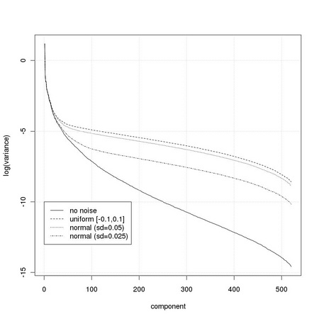
The required number of principal components depends on the specific task considered, and on the required performance. In some cases, the appropriate number can be determined by inspection of the values of the variance captured by the different directions. One such a case is that of images corrupted by noise. Usually, in the case of patterns not corrupted by noise, the variance associated to the different directions decreases quickly. When noise is present, i.e. white noise, its contribution may dominate the lowest variance directions. This is particularly evident for white noise, characterized by a constant variance for all directions, due to its spherical distribution. We are then interested in determining the cross point at which the contribution of the signal starts to be dominated by the noise.

We generate a set of pure noise images using two different types of noise: uniform and normal.

1 nu <- array(runif(800*525, min=-0.1,max=0.1), dim=c(800,525)) 
2 ng <- array(rnorm(800*525, sd=0.05), dim=c(800,525))

We can now perform PCA separately on the set of images corrupted by uniform noise

1 uSamples <- raceSamples1 + nu 
2 mycovU   <- cov(uSamples) 
3 mysvdU   <- fast.svd(mycovU)

and on the set of images corrupted by normal noise with a standard deviation of 0.05

1 gSamples <- raceSamples1 + ng 
2 mycovG   <- cov(gSamples) 
3 mysvdG   <- fast.svd(mycovG)

and with a standard deviation of 0.025

1 gSamples2 <- raceSamples1 + ng/2 
2 mycovG2   <- cov(gSamples2) 
3 mysvdG2   <- fast.svd(mycovG2)
1 tm.dev("figures/pca2", height=4.5) 
2 plot(log(mysvd1$d[1:520]), type="l", lty=1, xlab="component", ylab="log(variance)") 
3 lines(log(mysvdU$d[1:520]), lty=2) 
4 lines(log(mysvdG$d[1:520]),    lty=3) 
5 lines(log(mysvdG2$d[1:520]), lty=4) 
6 grid() 
7 legend(0,-10, c("no noise", "uniform [-0.1,0.1]", 
8 ...                 "normal (sd=0.05)", "normal (sd=0.025)"), 
9 ...        lty=c(1,2,3,4)) 
10 dev.off()

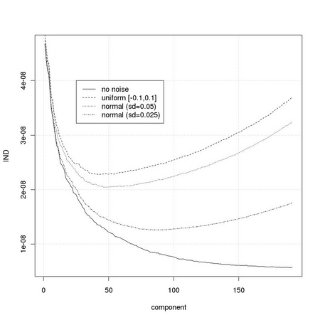
Let us define a simple indicator function following the description of Section TM8.1.2

1   tm.indf <- function(ls, d, N){ 
2 ...     vs <- array(0, dim=c(d)) 
3 ...     for(k in 1:d) { 
4 ...       s <- 0 
5 ...       for(j in (k+1):d) { 
6 ...         s <- s + ls[k] 
7 ...       } 
8 ...       vs[k] <- sqrt(s/(N*(d-k)))*(1/((d-k)*(d-k))) 
9 ...     } 
10 ...     vs 
11 ... }

and apply it to the eigenvalues sets just computed:

1   tm.dev("figures/pca3",  height=4.5) 
2   plot(tm.indf(mysvd1$d, 450, 800)[10:200],   type="l", lty=1, xlab="component", 
3 ...        ylab="IND") 
4   lines(tm.indf(mysvdU$d, 450, 800)[10:200],  lty=2) 
5   lines(tm.indf(mysvdG$d, 450, 800)[10:200],  lty=3) 
6   lines(tm.indf(mysvdG2$d, 450, 800)[10:200], lty=4) 
7   grid() 
8   legend(25,4e-8, c("no noise", "uniform [-0.1,0.1]", 
9 ...                     "normal (sd=0.05)", "normal (sd=0.025)"), 
10 ...          lty=c(1,2,3,4)) 
11   dev.off()


PICPIC

Figure 8.3: Increasing amounts of noise modify the eigenvalue distribution and anticipate the cross over point of the signal to noise ratio: the trend is correctly modeled by the minimum of the indicator function.