Fondazione Bruno Kessler - Technologies of Vision

contains material from
Template Matching Techniques in Computer Vision: Theory and Practice
Roberto Brunelli © 2009 John Wiley & Sons, Ltd

8.2 James-Stein estimation

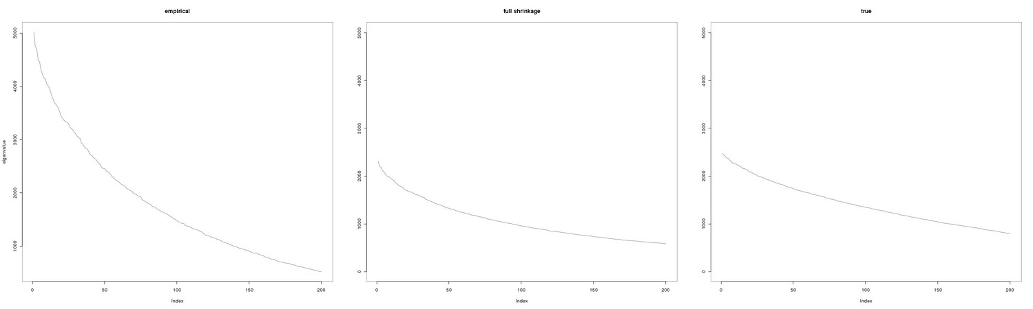
It may be worthwile to perform a simple simulation to check the potential advantage of using non standard estimators for the covariance matrix, the key quantity in PCA, in the case of large dimensionality and small number of samples.

1   # small n, large p 
2   # 
3   p <- 625 ;  n <- 400 
4   # 
5   # generate random pxp covariance matrix 
6   # 
7   sigma <- matrix(rnorm(p*p),ncol=p) 
8   sigma <- crossprod(sigma)+ diag(rep(0.01, p)) 
9   # 
10   # simulate multinormal data of sample size n 
11   # 
12   sigsvd <- svd(sigma) 
13   Y      <- t(sigsvd$v %*% (t(sigsvd$u) * sqrt(sigsvd$d))) 
14   X      <- matrix(rnorm(n * ncol(sigma)), nrow = n) %*% Y

Having generated our data sample we compute the covoriance matrix using the usual sample estimator and the shrinkage estimator:

1   sSample    <- cov(X) 
2   sShrinkage <- cov.shrink(X)

and proceed to the computation of the eigenvalues:

1   eTrue      <- eigen(sigma,      symmetric=TRUE)$values 
2   eSample    <- eigen(sSample,    symmetric=TRUE)$values 
3   eShrinkage <- eigen(sShrinkage, symmetric=TRUE)$values 
4   m          <-max(eTrue, eSample, eShrinkage) 
5   yl         <- c(0, m)

As reported in Figure 8.4, the advatange of shrinkage estimators over the standard ones can be dramatic.

1   tm.dev("figures/pca4", width=15) 
2   par(mfcol=c(1,3),lwd=0.5) 
3   plot(eSample[1:200],  main="empirical",ylab="eigenvalue", type="l") 
4   plot(eShrinkage[1:200],  ylim=yl, main="full shrinkage",ylab="", type="l") 
5   plot(eTrue[1:200],  ylim=yl, main="true",ylab="", type="l") 
6   grid(lwd=0.1) 
7   dev.off()


PIC

Figure 8.4: A good estimate of the covariance matrix is key to perform meaningful PCA. While the MLE sample estimate is commonly employed, it is far from optimal in the high dimensionality/few samples case.