|
Fondazione Bruno Kessler - Technologies of Vision
contains material from
Template Matching Techniques in Computer Vision: Theory and Practice
Roberto Brunelli © 2009 John Wiley & Sons, Ltd
Digital images are affected by characteristic artifacts that may impact significantly on template matching. We will consider two of them: demosaicing and interlacing.
High quality color imaging requires the sampling of three spectral bands at the same position and at the same time. While solutions exist the most common setup is based on a trick: a lattice of pixels, whose over number corresponds to the sensor resolution, is split into three different groups. The pixels of each group are covered with a small color filter. The result is that spectral information is not spatially aligned: each pixel only has information on one color. Full color information must then be recovered using interpolation techniques and the result is different from what would be obtained with full resolution color imaging especially in the proximity of color discontinuities.
|
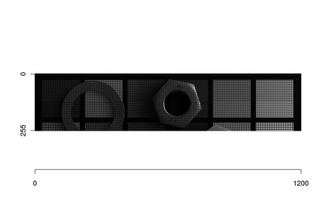
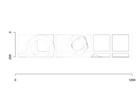
In some cases, image sensor data do not correspond to the same instant. Image rows are subdivided into two disjoint sets, each of them representing a field: all the rows of a single field share the same time but the two fields correspond to different instants. If the sensor is stationary and the scene is static a single image can be reconstructed by collating the two fields. If the camera is moving, or the scene is not static, the single image resulting from the integration of two fields exhibits noticeable artifacts.
Codelet 3 Interlaced image generation (../TeMa/R/tm.interlaceImage.R)
____________________________________________________________________________________________________________
Interlaced images are built by juxtaposition of two fields, each providing a partial image representation. This function simulates the generation of a full resolution image from two different fields with user selectable field distance specified by delta.
We get the field composed by the odd lines
and the one by the even lines
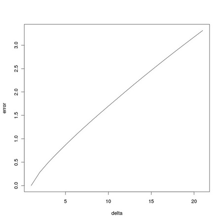
We can simulate different time lapse factors by changing the value of delta and translating one of the fields accordingly:
The full resolution image is simply obtained by summing the two fields:
A value delta=0 corresponds to a static scene and stationary camera and is equivalent to the output of a progressive sensor:
______________________________________________________________________________________
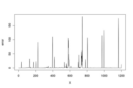
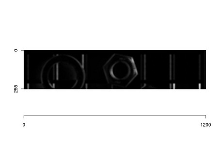
Interlacing impacts on template matching: line offset results in image differences that are not compensated by the matching process. As the following code snippet shows, the effect increases with the time delta of the two image fields and with the amount of local image structure (edges are the major sources of difference).
|