|
Fondazione Bruno Kessler - Technologies of Vision
contains material from
Template Matching Techniques in Computer Vision: Theory and Practice
Roberto Brunelli © 2009 John Wiley & Sons, Ltd
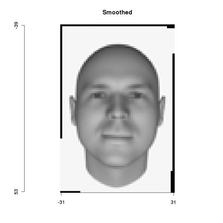
Image processing algorithms, template matching techniques included, often require image scaling and rotation. These operations are a subset of the linear transformations described by Equation TM:2.74. As an illustrative example let us consider geometric normalization of a face image: a combined rotation, scaling, and translation operation fixing the origin of the image coordinate system at the midpoint of the segment joining the eyes, at the same time making the eye to eye axis horizontal with eyes at a predefined distance from the new origin.
Image transformations of the type considered usually require image values at positions different from those of the original sampling. The computation of the new values can be performed correctly if the requirements of the sampling theorem are satisfied, sometimes requiring a preliminary smoothing step in order to reduce image frequency content, e.g. when reducing image size. The actual resampling operation can then be performed relying on Lanczos interpolation.
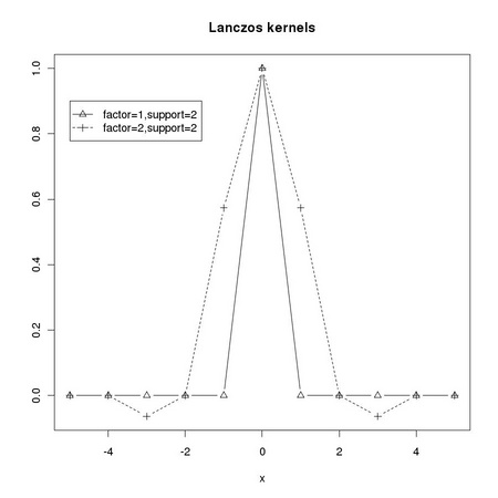
The frequency conditioning step can be performed applying a Gaussian smoothing kernel or a Lanczos kernel. Let us consider halving image resolution. As the Gaussian filter is approximately band limited with critical spacing σ and corresponding bad-limit σ-1∕2, it is appropriate to smooth the image with a σ = 2 Gaussian kernel (as we want to halve its resolution. If we use a Lanczos kernel we can rely on Equations TM:2.77-78 and sample the original kernel (twice) more densely. A function is available for computing the kernel, tm.lanczosKernel: the sampling density of the kernel is controlled by parameter factor.
If trim is omitted (or set to TRUE) the size of the kernel is appropriately computed to cover its support. Kernel lk22 is the one to use in preconditioning image frequency content prior to subsampling.
|